Introduction to NumPy
Contents
8. Introduction to NumPy#
The content of this section is derived from the book “Python data science hanbdbook”. Details of this book can be found in the further reading section.
NumPy is a scientific computing library and is the defacto library for numerical analysis and linear algebra in python i.e. it is “__Nu__merical __Py__thon”. It is a bit like Matlab for python. One of its primary features is the provision of efficient array data structures which are not particularly well supported in base python.
8.1. Arrays using Python Lists#
An array like structure can be created in python using lists.
8.1.1. Example 1#
A = [[1,2,3],[4,5,6],[7,8,9],[10,11,12]]
print(A)
[[1, 2, 3], [4, 5, 6], [7, 8, 9], [10, 11, 12]]
A[1][2]
6
In python, arrays represented as lists or, in the multidimensianal setting, lists of lists of lists …, have the advantage of being inhomogenous. However, when compared to arrays in other languages (which are commonly homogenous), they are not very efficient for random access.
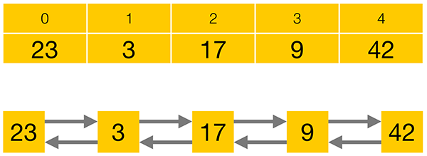
The following diagram shows a one dimensional array and the equivalent one dimensional list. Because an array is contiguous in memory, (no gaps in between successive data elements) it is possible to access the data very quickly using simple arithmetic. However, in a list, to get to value 17, you would have to start at 23 and march forward 2 places visiting 3 on the way. As the list grows, this repeated starting at the beginning and moving on becomes very expensive.
Python does come with an array type, but it is not particularly easy to use and is not well optimized for some of the more common array like operations.
array
 list
list
8.2. NumPy arrays#
Installing numpy.
! python -m pip install numpy
Requirement already satisfied: numpy in /home/grosedj/work/work-env/env/lib/python3.9/site-packages (1.23.2)
WARNING: You are using pip version 21.2.4; however, version 23.3.2 is available.
You should consider upgrading via the '/home/grosedj/work/work-env/env/bin/python -m pip install --upgrade pip' command.
Importing the numpy package (note the use of an the “alias” np).
import numpy as np
8.2.1. Exercise 1#
Install and import the numpy package.
8.3. Why NumPy Instead Of Python Lists?#
In general, there seem to be four possible reasons to prefer NumPy arrays over lists in Python:
NumPy arrays are more compact than lists.
access in reading and writing items is faster with NumPy.
NumPy can be more convenient to work with, thanks to the fact that you get a lot of vector and matrix operations for free
NumPy can be more efficient to work with because they are implemented more efficiently.
8.4. Creating and acessing NumPy arrays#
8.4.1. Example 2 - creating NumPy array from a list#
X = np.array([[1,2,3],[4,5,6]])
print(X)
[[1 2 3]
 [4 5 6]]
8.4.2. Exercise 2 - indexing tnto a NumPy array#
What do you think the output of the following code will be ?
print(X[1,0])
print(X[1])
print(X[1][0])
X[0,2] = 10
print(X)
4
[4 5 6]
4
[[ 1  2 10]
 [ 4  5  6]]
8.4.3. Exercise 3#
Use help function to find out about the following functions that can be used for initialising NumPy arrays.
ones
zeros
empty
help(np.empty)
Help on built-in function empty in module numpy:

empty(...)
    empty(shape, dtype=float, order='C', *, like=None)

    Return a new array of given shape and type, without initializing entries.

    Parameters
    ----------
    shape : int or tuple of int
        Shape of the empty array, e.g., ``(2, 3)`` or ``2``.
    dtype : data-type, optional
        Desired output data-type for the array, e.g, `numpy.int8`. Default is
        `numpy.float64`.
    order : {'C', 'F'}, optional, default: 'C'
        Whether to store multi-dimensional data in row-major
        (C-style) or column-major (Fortran-style) order in
        memory.
    like : array_like, optional
        Reference object to allow the creation of arrays which are not
        NumPy arrays. If an array-like passed in as ``like`` supports
        the ``__array_function__`` protocol, the result will be defined
        by it. In this case, it ensures the creation of an array object
        compatible with that passed in via this argument.

        .. versionadded:: 1.20.0

    Returns
    -------
    out : ndarray
        Array of uninitialized (arbitrary) data of the given shape, dtype, and
        order.  Object arrays will be initialized to None.

    See Also
    --------
    empty_like : Return an empty array with shape and type of input.
    ones : Return a new array setting values to one.
    zeros : Return a new array setting values to zero.
    full : Return a new array of given shape filled with value.


    Notes
    -----
    `empty`, unlike `zeros`, does not set the array values to zero,
    and may therefore be marginally faster.  On the other hand, it requires
    the user to manually set all the values in the array, and should be
    used with caution.

    Examples
    --------
    >>> np.empty([2, 2])
    array([[ -9.74499359e+001,   6.69583040e-309],
           [  2.13182611e-314,   3.06959433e-309]])         #uninitialized

    >>> np.empty([2, 2], dtype=int)
    array([[-1073741821, -1067949133],
           [  496041986,    19249760]])                     #uninitialized
8.4.4. Exercise 4 - creating a NumPy array from scratch#
Create a three dimensional numpy array with dimension 3,5,2 that contains floating point numbers. What do the contents look like ? How does this compare with using zeros ? How you create the same array but for use with integer values ?
X = np.empty((3,5,2))
print(X[0])
X = np.empty((3,5,2),dtype="int")
print(X[0])
[[4.67592250e-310 0.00000000e+000]
 [4.67648006e-310 0.00000000e+000]
 [0.00000000e+000 0.00000000e+000]
 [4.94065646e-324 5.20521812e+223]
 [4.19338351e+228 0.00000000e+000]]
[[ 94641744298500               0]
 [140290495184816 140290496109296]
 [140290495589952 140290468620928]
 [140290468621008 140290468621088]
 [140290468607168 140290494606832]]
NumPy has many more basic types of data than base python. They typically map to the basic C types that they are built on.
Numpy type |
C type |
Description |
|---|---|---|
|
Boolean (True or False) stored as a byte |
|
|
Platform-defined |
|
|
Platform-defined |
|
|
Platform-defined |
|
|
Platform-defined |
|
|
Platform-defined |
|
|
Platform-defined |
|
|
Platform-defined |
|
|
Platform-defined |
|
|
Platform-defined |
|
|
Platform-defined |
|
Half precision float: sign bit, 5 bits exponent, 10 bits mantissa |
||
|
Platform-defined single precision float: typically sign bit, 8 bits exponent, 23 bits mantissa |
|
|
Platform-defined double precision float: typically sign bit, 11 bits exponent, 52 bits mantissa. |
|
|
Platform-defined extended-precision float |
|
|
Complex number, represented by two single-precision floats (real and imaginary components) |
|
|
Complex number, represented by two double-precision floats (real and imaginary components). |
|
|
Complex number, represented by two extended-precision floats (real and imaginary components). |
8.5. Slicing and accessing subarrays#
Subarrays can be access using the format [start:stop:step].
8.5.1. Example 3 - slicing#
X = np.array([[1,2,3,4],[5,6,7,8],[9,10,11,12],[13,14,15,16]])
print(X[0:2:1])
[[1 2 3 4]
 [5 6 7 8]]
8.5.2. Exercise 5#
Predict the output of the following code.
print(X[0:3:2])
[[ 1  2  3  4]
 [ 9 10 11 12]]
print(X[0:3:1][:2:1])
[[1 2 3 4]
 [5 6 7 8]]
print(X[0:3:1][:2:2])
[[1 2 3 4]]
print(X[:3:][:2:2])
[[1 2 3 4]]
print(X[:3:,:2:2])
[[1]
 [5]
 [9]]
print(X[::2,::2])
[[ 1  3]
 [ 9 11]]
print(X[1:3:,1:3:])
[[ 6  7]
 [10 11]]
print(X[:,1])
[ 2 6 10 14]
print(X[1,:])
[5 6 7 8]
Z = X[1:3:,1:3:]
Z[1,1] = 20
print(X)
[[ 1  2  3  4]
 [ 5  6  7  8]
 [ 9 10 20 12]
 [13 14 15 16]]
Note that in the last example, Z is NOT a copy of the data inside X, it is a “view” on the data contained in X. You can create a copy using copy.
8.5.3. Example 4 - copying#
Z = X[1:3:,1:3:].copy()
Z[1,1] = 50
print(X)
print(Z)
[[ 1  2  3  4]
 [ 5  6  7  8]
 [ 9 10 20 12]
 [13 14 15 16]]
[[ 6  7]
 [10 50]]
8.5.4. Exercise 6#
Use help to find out how to use the NumPy reshape, concatenate, vstack, and hstack functions.
help(np.concatenate)
Help on function concatenate in module numpy:

concatenate(...)
    concatenate((a1, a2, ...), axis=0, out=None, dtype=None, casting="same_kind")

    Join a sequence of arrays along an existing axis.

    Parameters
    ----------
    a1, a2, ... : sequence of array_like
        The arrays must have the same shape, except in the dimension
        corresponding to `axis` (the first, by default).
    axis : int, optional
        The axis along which the arrays will be joined.  If axis is None,
        arrays are flattened before use.  Default is 0.
    out : ndarray, optional
        If provided, the destination to place the result. The shape must be
        correct, matching that of what concatenate would have returned if no
        out argument were specified.
    dtype : str or dtype
        If provided, the destination array will have this dtype. Cannot be
        provided together with `out`.

        .. versionadded:: 1.20.0

    casting : {'no', 'equiv', 'safe', 'same_kind', 'unsafe'}, optional
        Controls what kind of data casting may occur. Defaults to 'same_kind'.

        .. versionadded:: 1.20.0

    Returns
    -------
    res : ndarray
        The concatenated array.

    See Also
    --------
    ma.concatenate : Concatenate function that preserves input masks.
    array_split : Split an array into multiple sub-arrays of equal or
                  near-equal size.
    split : Split array into a list of multiple sub-arrays of equal size.
    hsplit : Split array into multiple sub-arrays horizontally (column wise).
    vsplit : Split array into multiple sub-arrays vertically (row wise).
    dsplit : Split array into multiple sub-arrays along the 3rd axis (depth).
    stack : Stack a sequence of arrays along a new axis.
    block : Assemble arrays from blocks.
    hstack : Stack arrays in sequence horizontally (column wise).
    vstack : Stack arrays in sequence vertically (row wise).
    dstack : Stack arrays in sequence depth wise (along third dimension).
    column_stack : Stack 1-D arrays as columns into a 2-D array.

    Notes
    -----
    When one or more of the arrays to be concatenated is a MaskedArray,
    this function will return a MaskedArray object instead of an ndarray,
    but the input masks are *not* preserved. In cases where a MaskedArray
    is expected as input, use the ma.concatenate function from the masked
    array module instead.

    Examples
    --------
    >>> a = np.array([[1, 2], [3, 4]])
    >>> b = np.array([[5, 6]])
    >>> np.concatenate((a, b), axis=0)
    array([[1, 2],
           [3, 4],
           [5, 6]])
    >>> np.concatenate((a, b.T), axis=1)
    array([[1, 2, 5],
           [3, 4, 6]])
    >>> np.concatenate((a, b), axis=None)
    array([1, 2, 3, 4, 5, 6])

    This function will not preserve masking of MaskedArray inputs.

    >>> a = np.ma.arange(3)
    >>> a[1] = np.ma.masked
    >>> b = np.arange(2, 5)
    >>> a
    masked_array(data=[0, --, 2],
                 mask=[False,  True, False],
           fill_value=999999)
    >>> b
    array([2, 3, 4])
    >>> np.concatenate([a, b])
    masked_array(data=[0, 1, 2, 2, 3, 4],
                 mask=False,
           fill_value=999999)
    >>> np.ma.concatenate([a, b])
    masked_array(data=[0, --, 2, 2, 3, 4],
                 mask=[False,  True, False, False, False, False],
           fill_value=999999)
The shape of a NumPy array can be found quite easily.
  Cell In [22], line 1
    The shape of a NumPy array can be found quite easily.
        ^
SyntaxError: invalid syntax
print(X.shape)
(4, 4)
8.6. Random numbers.#
The NumPy library is more than an array library. For example, it offers random number generation.
8.6.1. Example 5 - uniform random numbers#
np.random.rand(3,2)
array([[0.3150833 , 0.33404232],
       [0.44625496, 0.54454593],
       [0.56114458, 0.14973511]])
8.6.2. Exercise 7#
Use help(np.random)) to find out about random number generation in NumPy. Generate large matrices of random numbers from some of these distributions.
help(np.random.rand)
Help on built-in function rand:

rand(...) method of numpy.random.mtrand.RandomState instance
    rand(d0, d1, ..., dn)

    Random values in a given shape.

    .. note::
        This is a convenience function for users porting code from Matlab,
        and wraps `random_sample`. That function takes a
        tuple to specify the size of the output, which is consistent with
        other NumPy functions like `numpy.zeros` and `numpy.ones`.

    Create an array of the given shape and populate it with
    random samples from a uniform distribution
    over ``[0, 1)``.

    Parameters
    ----------
    d0, d1, ..., dn : int, optional
        The dimensions of the returned array, must be non-negative.
        If no argument is given a single Python float is returned.

    Returns
    -------
    out : ndarray, shape ``(d0, d1, ..., dn)``
        Random values.

    See Also
    --------
    random

    Examples
    --------
    >>> np.random.rand(3,2)
    array([[ 0.14022471,  0.96360618],  #random
           [ 0.37601032,  0.25528411],  #random
           [ 0.49313049,  0.94909878]]) #random
X = np.random.rand(1000,1000)
print(X[1:10,1:10])
[[0.93725918 0.06203331 0.83580012 0.03160988 0.7798329  0.30640705
  0.7414987  0.99160143 0.14266476]
 [0.95206452 0.14178445 0.09118578 0.17457443 0.76104316 0.28949847
  0.29942323 0.07608373 0.05289887]
 [0.25530272 0.66924424 0.28340527 0.71735581 0.30488826 0.30623068
  0.47408782 0.70436219 0.58647558]
 [0.26812957 0.87237088 0.51070945 0.53435651 0.73995196 0.75998788
  0.58319684 0.65992788 0.70158033]
 [0.24103802 0.19956387 0.74662767 0.84646724 0.12328907 0.26932249
  0.38748918 0.72313705 0.40867608]
 [0.63366512 0.05276984 0.1132461  0.08810961 0.320329   0.31010316
  0.64176265 0.22798977 0.95000039]
 [0.45652143 0.00195218 0.2580788  0.87617122 0.41812466 0.96003646
  0.85651487 0.51288647 0.98163307]
 [0.7487736  0.90593057 0.34325887 0.79687955 0.57725936 0.76379036
  0.73959716 0.75815155 0.50633209]
 [0.60686795 0.98670865 0.01420011 0.23918258 0.77386063 0.12878113
  0.37959095 0.14720258 0.7509649 ]]
8.6.3. Exercise 8#
Write a function that calculates the sine of each value one of the large matrices you generated for excercise 7.
from math import sin
def matsin(X) :
    (n,m) = X.shape
    Y = np.empty((n,m))
    for i in range(n) :
        for j in range(m) :
            Y[i,j] = sin(X[i,j])
    return(Y)

Y = matsin(X)
print(Y[1:10,1:10])
[[0.80593856 0.06199353 0.7418333  0.03160461 0.70316061 0.30163499
  0.6753939  0.8369036  0.14218131]
 [0.81461467 0.14130988 0.09105946 0.17368905 0.68967719 0.2854716
  0.29496915 0.07601035 0.0528742 ]
 [0.25253833 0.62039343 0.27962669 0.65739445 0.30018659 0.30146683
  0.45652706 0.64754793 0.55342899]
 [0.26492831 0.76585559 0.48879629 0.50928736 0.67425243 0.68891266
  0.55069517 0.61305988 0.64542558]
 [0.23871077 0.19824188 0.67916739 0.74894416 0.12297697 0.26607841
  0.37786494 0.66173988 0.39739478]
 [0.59210231 0.05274536 0.1130042  0.08799565 0.31487884 0.30515688
  0.59860833 0.22601977 0.81341573]
 [0.44082845 0.00195218 0.25522345 0.76829373 0.40604739 0.81921248
  0.75556414 0.49069436 0.83140592]
 [0.6807409  0.78699961 0.33655763 0.71517857 0.54572944 0.69166388
  0.67399037 0.68758045 0.48497282]
 [0.57029747 0.83421552 0.01419964 0.23690855 0.69890163 0.12842546
  0.37054057 0.14667154 0.68234445]]
It is possibe to measure how long code takes to run using %timeit.
8.6.4. Example 6 - %timeit#
%timeit matsin(X)
250 ms ± 6.47 ms per loop (mean ± std. dev. of 7 runs, 1 loop each)
8.7. NumPy UFuncs#
NumPy’s ufuncs can be used to make repeated calculations on array elements much more efficient. ufuncs apply use vectorization to undertake large numbers of operations using fast compiled C code without having to call the underlying C functions repeatedly. This can make things much faster.
8.7.1. Exercise 9#
Use %timeit to find out how long the following python code takes to run. Compare it to the reuslts you obtained from exercise 8.
%timeit Y = np.sin(X)
8.88 ms ± 112 µs per loop (mean ± std. dev. of 7 runs, 100 loops each)
There are lots of ufuncs in NumPy. They include various operators for example.
8.7.2. Example 7#
Y = X + X
Y = 2*X
Y = X*X
Note that the * is NOT matrix multiplication. For this you have to use the matmul function.