
8. Session 6 : Data Structures - Computational Complexity#
8.1. Session Overview#
The objectives of this session are
Understand datastructures in a declarative sense as mappings between sets
Understand computational complexity in terms of asymptotics
Understand the difference between several common asymptotic measures of computational complexity
Understand the difference between best, worst, and average cases
Know the basic data structures provided by python and what mappings they correspond to, and how to use them
Know the computational complexity of popular python implementations of common data structures
Know how to choose data structures according to use case
8.2. Data structures as mappings#
At a useful level of abstraction, a data structure is a way of representing and organizing data so that certain operations can be performed efficiently.
Most data structures can be viewed as implementations of one or more mathematical mappings between sets.
At minimum, a data structure represents a (possibly partial) function
where \(K\) is a set of keys (indices, positions, labels, states) and \(V\) is a set of values.
8.2.1. Examples#
Arrays / vectors: a mapping from a finite index set \(\{0,\dots,n-1\}\) to values.
Hash tables / dictionaries: a mapping from an arbitrary key set to values, typically approximating constant-time access.
Trees and graphs: mappings from nodes to collections of nodes (adjacency), or from keys to values with additional structural constraints.
Matrices and tensors: mappings from multi-dimensional index tuples to values.
What distinguishes data structures is not the mapping itself, but the constraints imposed on how the mapping is stored and traversed (ordering, hierarchy, sparsity, locality).
8.2.2. Operations and abstract interfaces#
Each data structure supports a set of operations that correspond to queries or transformations of the mapping:
lookup: evaluate \(f(k)\)
insert / delete: modify the domain or codomain
iterate: traverse the domain in a prescribed order
aggregate: compute functions over subsets of the mapping
Formally, a data structure can be seen as an algorithmic representation of an abstract data type (ADT): a set plus a collection of operations with specified semantics.
8.2.3. Computational complexity as the defining trade-off#
The central purpose of a data structure is to control the computational complexity of these operations.
Complexity is typically measured asymptotically in terms of:
time (e.g. \(O(1), O(\log n), O(n)\))
space (memory usage as a function of input size)
Different data structures represent the same abstract mapping but optimize different operations.
8.2.4. Examples of trade-offs#
An array gives \(O(1)\) access by index but \(O(n)\) insertion.
A balanced binary search tree gives \(O(\log n)\) lookup, insertion, and deletion while maintaining order.
A hash table sacrifices ordering to achieve expected \(O(1)\) lookup.
Choosing a data structure is therefore equivalent to choosing a complexity profile over a set of operations.
8.2.5. Summary#
Data structures mediate between mathematical objects (functions, relations, graphs, tensors) and computational reality (finite memory, cache behavior, parallelism).
They determine whether an algorithm is feasible at scale, not just correct.
Many performance bottlenecks arise not from the algorithmic idea, but from a mismatch between the structure of the data and the structure imposed by the data structure.
In short: a data structure is a concrete, complexity-aware realization of a mapping, designed to make specific operations fast while accepting trade-offs elsewhere.
8.3. Computational Complexity#
Computational complexity studies how the resources required by an algorithm scale with the size of the input. The two dominant resources are:
Time complexity: number of elementary operations executed
Space complexity: amount of memory used
Formally, if an algorithm takes an input of size ( n ), its time complexity is a function
\(T(n) = \text{number of steps executed on inputs of size } n.\)
The key idea is scaling behavior, not exact runtime. Complexity theory abstracts away:
hardware details,
constant factors,
implementation quirks,
and focuses on growth rates as \( n \to \infty \).
This is important because :
datasets grow,
asymptotic behavior dominates practical feasibility,
algorithm choice often beats micro-optimisation by orders of magnitude.
8.3.1. Asymptotic analysis#
8.3.1.1. Big-O notation (upper bounds)#
We say \(T(n) \in O(f(n))\) if there exist constants \( c > 0 \) and \( n_0 \) such that \(T(n) \le c f(n) \quad \forall n \ge n_0\).
Interpretation:
\( f(n) \) is an asymptotic upper bound on the algorithm’s growth.
Example:
\(T(n) = 3n^2 + 5n + 20 \in O(n^2)\).
8.3.1.2. Big-Ω notation (lower bounds)#
\( T(n) \in \Omega(f(n)) \quad \Longleftrightarrow \quad T(n) \ge c f(n) \text{ eventually}. \)
This gives a guaranteed minimum growth rate.
8.3.1.3. Big-Θ notation (tight bounds)#
\( T(n) \in \Theta(f(n)) \quad \Longleftrightarrow \quad T(n) \in O(f(n)) \cap \Omega(f(n)). \)
This means \( f(n) \) characterises the true asymptotic order.
8.3.1.4. Overview#
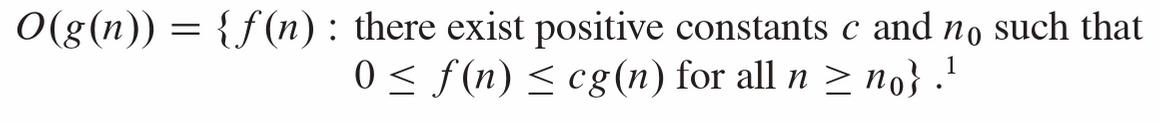

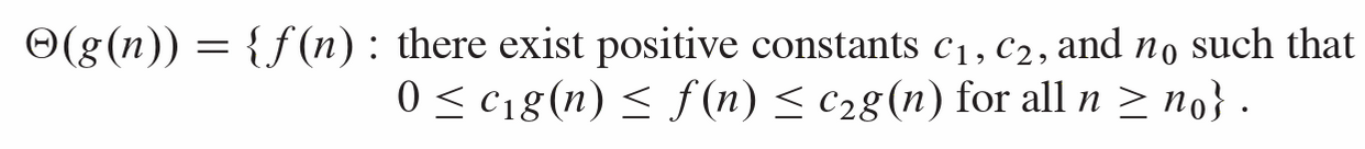
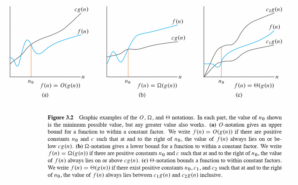
The above definitions and figure are taken from Intoduction to Algorithms
In practice, Big-O is most commonly used, even when tighter bounds exist.
8.3.2. Best case, worst case, and average case#
An algorithm’s runtime may depend not just on input size \( n \), but on the structure of the input. We therefore distinguish cases.
8.3.2.1. Worst-case complexity#
\( T_{\text{worst}}(n) = \max_{\text{inputs}} T(\text{input}) \) where all of the iputs are of size \(n\).
Provides a guarantee
Common in algorithm analysis and systems design
Often pessimistic but robust
Example:
Linear search in an unsorted array
Worst case: element not present → ( O(n) )
8.3.2.2. Best-case complexity#
\( T_{\text{best}}(n) = \min_{\text{inputs}} T(\text{input}) \) where all of the iputs are of size \(n\).
Rarely used alone
Can be misleading
Useful when best-case happens frequently or is structurally meaningful
Example:
Linear search: target is first element → ( O(1) )
8.3.2.3. Average-case complexity#
\( T_{\text{avg}}(n) = \mathbb{E}[T(X_n)] \) where \( X_n \) is a random input of size \( n \) drawn from some probability distribution.
Average case is only meaningful relative to an assumed input distribution.
Example:
Quicksort:
Worst case: ( O(n^2) )
Average case (under random permutations): \( \Theta(n \log n) \)
Importantly, This connects naturally to:
probabilistic modelling of data,
assumptions about randomness,
distribution-sensitive algorithms.
8.3.2.4. Amortised analysis: averaging over sequences, not inputs#
Amortised complexity analyzes the average cost per operation over a sequence of operations, even if individual operations are expensive.
Crucially :
No probability is involved
Guarantees hold for every sequence
Let a sequence of \( m \) operations take total time \( T(m) \).
The amortised cost per operation is:
\(
\frac{T(m)}{m}.
\)
8.4. Computational Complexity of Common Python Data Structures#
8.4.1. list#
Operation |
Time |
|---|---|
Index access |
O(1) |
Append |
O(1) amortized |
Pop end |
O(1) |
Insert / delete middle |
O(n) |
Membership |
O(n) |
Sort |
O(n log n) |
8.4.2. dict#
Operation |
Time |
|---|---|
Lookup |
O(1) avg |
Insert / update |
O(1) avg |
Delete |
O(1) avg |
Membership |
O(1) avg |
Iterate |
O(n) |
Worst-case O(n) (hash collisions, rare)
8.4.3. set#
Operation |
Time |
|---|---|
Add |
O(1) avg |
Remove |
O(1) avg |
Membership |
O(1) avg |
Union / intersect |
O(n) |
8.4.4. deque#
Operation |
Time |
|---|---|
Append right / left |
O(1) |
Pop right / left |
O(1) |
Index access |
O(n) |
Insert / delete middle |
O(n) |
Best for queues, BFS, sliding windows
8.4.5. namedtuple#
Operation |
Time |
|---|---|
Field access |
O(1) |
Index access |
O(1) |
Creation |
O(n) |
Mutation |
❌ (immutable) |
Same performance as
tuple, just nicer syntax
8.4.6. SortedList#
Operation |
Time |
|---|---|
Index access |
O(1) |
Insert |
O(log n) |
Delete |
O(log n) |
Membership |
O(log n) |
Bisect |
O(log n) |
8.4.7. SortedDict#
Operation |
Time |
|---|---|
Lookup |
O(log n) |
Insert |
O(log n) |
Delete |
O(log n) |
Min / max key |
O(1) |
8.4.8. SortedSet#
Operation |
Time |
|---|---|
Add |
O(log n) |
Remove |
O(log n) |
Membership |
O(log n) |
Iterate (sorted) |
O(n) |
8.5. Exercises#
8.5.1. list#
8.5.1.1. Key ideas#
Ordered, mutable, allows duplicates
Fast append, slow insert/delete in the middle
8.5.1.2. Exercise 1 - Indexing and slicing#
data = [3, 5, 7, 11, 13, 17]
Extract the last three elements using slicing
Reverse the list using slicing (no loops)
What happens if you try to access
data[10]?
8.5.1.3. Exercise 2: Mutation#
Exercise 2: Mutation
data = [10, 20, 30]
Append
40Insert
15at index1Remove
20using two different methodsObserve the return values of
append,insert, andremove
8.5.1.4. Exercise 3: Performance intuition#
Time how long it takes to:
append()100,000 itemsinsert(0, x)100,000 items
Explain the difference.
8.5.1.5. Use cases#
Storing raw observations
Feature vectors
Sequential data (time series before indexing)
Mini-batches during model training
8.5.2. tuple#
8.5.2.1. Key ideas#
Ordered, immutable
Hashable (if contents are hashable)
8.5.2.2. Exercise 1: Immutability#
point = (3, 4)
Try changing
point[0]Create a new tuple with
xdoubled
8.5.2.3. Exercise 2: Tuple unpacking#
record = ("Alice", 22, "Biology")
Unpack into three variables
Swap two variables without using a temp variable
8.5.2.4. Exercise 3: Tuples as keys#
locations = {
    (40.7, -74.0): "New York",
    (34.0, -118.2): "Los Angeles"
}
Look up a city
Explain why lists can’t be used as keys
8.5.2.5. Use cases#
Fixed records (rows)
Coordinates (lat, long)
Dictionary keys for multi-dimensional indexing
Lightweight, memory-efficient records
8.5.3. set#
8.5.4. Key ideas#
Unordered, mutable
No duplicates
Fast membership tests
Exercise 1: Deduplication
ids = [101, 102, 101, 103, 102]
Convert to a set
Convert back to a list
What information was lost?
Exercise 2: Set operations*
A = {1, 2, 3, 4}
B = {3, 4, 5, 6}
Compute union, intersection, difference
Use both operators and methods
8.5.4.1. Exercise 3: Membership timing#
Time
x in listvsx in setfor large collectionsExplain why the set is faster
8.5.4.2. Use cases#
Unique identifiers
Feature vocabularies
Removing duplicates
Fast filtering and membership checks
8.5.5. dict#
8.5.5.1. Key ideas#
Key–value mapping
Insertion-ordered (Python ≥3.7)
Fast lookups
8.5.5.2. Exercise 1: Basic operations#
counts = {}
Count word frequencies from a list of strings
Rewrite using
dict.getRewrite using
collections.defaultdict
8.5.5.3. Exercise 2: Iteration#
data = {"A": 10, "B": 20, "C": 30}
Iterate over keys
Iterate over values
Iterate over key–value pairs
8.5.5.4. Exercise 3: Dictionary views#
Store
keys(),values(),items()in variablesModify the dictionary
Observe how the views change
8.5.5.5. Use cases#
Feature mappings
Label encoding
Aggregations
Sparse representations
8.5.6. str#
8.5.6.1. Key ideas#
Immutable sequence of characters
Rich API for text processing
8.5.6.2. Exercise 1: Indexing and slicing#
text = "Data Science"
Extract
"Science"Reverse the string
Get every second character
8.5.6.3. Exercise 2: String methods#
Convert to lowercase
Replace spaces with
_Split into words
8.5.6.4. Exercise 3: Immutability#
Try modifying a character
Create a modified copy instead
8.5.6.5. Use cases#
Text preprocessing
Tokenization
Feature extraction
Labels and metadata
8.5.7. deque#
8.5.7.1. Key ideas#
Double-ended queue
Fast appends and pops from both ends
8.5.7.2. Exercise 1: Basic operations#
from collections import deque
dq = deque([1, 2, 3])
Append to the right
Append to the left
Pop from both ends
8.5.7.3. Exercise 2: Sliding window#
Use a deque of max length 5
Simulate streaming data
Observe how old values are discarded
8.5.7.4. Exercise 3: Compare with list#
Time
pop(0)on a listTime
popleft()on a deque
8.5.7.5. Use cases#
Streaming data
Rolling averages
Buffers and queues
Time-windowed analytics
8.5.8. namedtuple#
8.5.8.1. Key ideas#
Tuple with named fields
Immutable
Lightweight alternative to classes
8.5.8.2. Exercise 1: Creation#
from collections import namedtuple
Student = namedtuple("Student", ["name", "age", "major"])
Create a student
Access fields by name and index
8.5.8.3. Exercise 2: Immutability#
Try modifying a field
Use
_replaceto create a new version
8.5.8.4. Exercise 3: Comparison#
Compare a
namedtupleto:tuple
dictionary
Discuss readability vs flexibility
8.5.8.5. Use cases#
Structured records
Configuration objects
Model outputs
Lightweight row representations
8.5.9. SortedList#
8.5.9.1. Key ideas#
Maintains sorted order automatically
Fast lookup and slicing
8.5.9.2. Exercise 1: Automatic sorting#
from sortedcontainers import SortedList
sl = SortedList()
Add numbers in random order
Observe ordering after each insert
8.5.9.3. Exercise 2: Indexing and slicing#
Access smallest and largest values
Slice the middle range
8.5.9.4. Exercise 3: Comparison#
Compare with:
sorting a list repeatedly
heapq
Discuss trade-offs
8.5.9.5. Use cases#
Online statistics
Maintaining quantiles
Ranked scores
Real-time leaderboards
8.5.10. SortedSet#
8.5.10.1. Key ideas#
Sorted + unique
Combines
setsemantics with order
8.5.10.2. Exercise 1: Deduplication + order#
from sortedcontainers import SortedSet
ss = SortedSet([5, 1, 3, 3, 2])
Observe ordering
Try adding duplicates
8.5.10.3. Exercise 2: Set operations#
Intersection and union with another
SortedSetCompare with regular
set
8.5.10.4. Data science use cases#
Unique sorted categories
Feature vocabularies with order
Ranked identifiers
8.5.11. SortedDict#
8.5.11.1. Key ideas#
Dictionary sorted by keys
Efficient range queries
8.5.11.2. Exercise 1: Ordered keys#
from sortedcontainers import SortedDict
sd = SortedDict()
Insert keys out of order
Iterate over keys and values
8.5.11.3. Exercise 2: Range queries#
Retrieve items with keys between two values
Compare with normal
dict
8.5.11.4. Use cases#
Time-indexed data
Ordered categorical mappings
Efficient range filtering
Event logs
8.5.12. Summary Exercise#
Which structures preserve order? Which don’t?
Which are mutable vs immutable?
When would sortedcontainers outperform built-in types?
Which data structures would you choose for:
Streaming data
Text analysis
Real-time rankings
Sparse features
8.6. Data Structure Choice#
8.6.1. Example 1#
You need to store a growing sequence of observations in arrival order
Choice: list
Why:
Preserves insertion order
Fast
append()→ O(1) amortizedSimple indexing and slicing
Why not others:
dequeis unnecessary unless removing from the frontSortedListadds overhead if order of arrival matters
8.6.2. Example 2#
You need a fixed record representing a row of data (name, age, major)
Choice: namedtuple
Why:
Immutable → safer for records
Clear, readable field access (
student.age)More memory-efficient than a dictionary
Why not others:
dictis flexible but less structuredtuplelacks readability
8.6.3. Example 3#
You need fast membership tests for millions of IDs
Choice: set
Why:
Average-case O(1) membership tests
Automatically removes duplicates
Why not others:
listmembership is O(n)SortedSetadds overhead if order is irrelevant
8.6.4. Example 4#
You need to count frequencies of categories or words
Choice: dict (or defaultdict)
Why:
Fast updates and lookups → O(1) average
Natural key → count mapping
Scales well for sparse data
Why not others:
listwould require searchingsetcannot store counts
8.6.5. Example 5#
You need to remove duplicates but also keep values sorted
Choice: SortedSet
Why:
Enforces uniqueness like a
setMaintains sorted order automatically
Efficient iteration in order
Why not others:
setis unorderedlistrequires manual sorting and duplicate removal
8.6.6. Example 6#
You need a rolling window over streaming data
Choice: deque
Why:
Fast insertion/removal at both ends → O(1)
Supports fixed-size windows
Designed for queue-like behavior
Why not others:
list.pop(0)is O(n)SortedListis unnecessary if only order matters
8.6.7. Example 7#
You need to compute rolling medians in real time
Choice: SortedList
Why:
Maintains sorted order on insertion → O(log n)
Median retrieval is O(1)
Ideal for online statistics
Why not others:
Sorting a list repeatedly is expensive
heapqis more complex for median logic
8.6.8. Example 8#
You need to store time-indexed data and query ranges
Choice: SortedDict
Why:
Keys always sorted
Efficient range queries
Natural fit for timestamps
Why not others:
Regular
dictrequires manual sortinglistloses key–value semantics
8.6.9. Example 9#
You need to store coordinates or multi-dimensional keys
Choice: tuple (as dictionary keys)
Why:
Immutable and hashable
Lightweight
Safe as dictionary keys
Why not others:
listis mutable and unhashabledictis unnecessary nesting
8.6.10. Example 10#
You need to preprocess and clean text data
Choice: str (with list/dict support)
Why:
Rich built-in API
Immutable → safe transformations
Works well with pipelines
Why not others:
listof characters is harder to manageMutability adds bugs without benefit
8.7. Summary#
8.7.1. Cheat Sheet#
Choose the simplest structure that
supports the required operations efficiently
matches the data’s mutability and ordering needs
minimizes unnecessary overhead
Need |
Best Choice |
|---|---|
Fast append |
|
Fast front removal |
|
Unique items |
|
Key → value |
|
Fixed record |
|
Sorted data |
|
Sorted + unique |
|
Sorted keys |
|