2. Data types and structures#
Some parts of this section have been copied from, or based on, material in the R programming wikibook.
2.1. Overview#
Most programming systems and languages have some basic data types which allow data to be represented, organised and accessed efficiently by programs written in the language. This section introduces some of the most common and useful data types available in the base R system. Note that there are many other types of data structure that could be useful for statistical programming and data manipulation which are not part of the base distribution of R. However, many of these other data structures are provided through packages that are available in the public domain. For example, the datastructures package.
2.2. Introduction#
Vectors are the simplest R objects, an ordered list of primitive R objects of a given type (e.g. real numbers, strings, logicals). Vectors are indexed by integers starting at 1. Factors are similar to vectors but where each element is categorical, i.e. one of a fixed number of possibilities (or levels). A matrix is like a vector but with a specific instruction for the layout such that it looks like a matrix, i.e. the elements are indexed by two integers, each starting at 1. Arrays are similar to matrices but can have more than 2 dimensions. A list is similar to a vector, but the elements need not all be of the same type. The elements of a list can be indexed either by integers or by named strings, i.e. an R list can be used to implement what is known in other languages as an “associative array”, “hash table”, “map” or “dictionary” - but not in a very efficient manner !! A dataframe is like a matrix but does not assume that all columns have the same type. A dataframe is a list of variables/vectors of the same length. Classes define how objects of a certain type look like. Classes are attached to object as an attribute. All R objects have a class, a type and a dimension. The class, type, and dimension of an object can be determined using the class, typeof, and dim functions.
x<-c(1,2,3,4)
Y<-matrix(c(1,2,3,4),2,2)
class(x)
typeof(x)
dim(x)
NULL
class(Y)
typeof(Y)
dim(Y)
- 'matrix'
- 'array'
- 2
- 2
2.3. Vectors#
You can create a vector using the c() function which concatenates some elements. You can create a sequence using the : symbol or the seq() function. For instance 1:5 gives all the number between 1 and 5. The seq() function lets you specify the interval between the successive numbers. You can also repeat a pattern using the rep() function. You can also create a numeric vector of missing values using numeric(), a character vector of missing values using character() and a logical vector of missing values (i.e. FALSE) using logical().
2.3.1. Exercise 1#
See if you can predict the output from each of these ways of creating vectors.
c(1,2,3,4,5)
Show code cell output
- 1
- 2
- 3
- 4
- 5
c("a","b","c","d","e")
Show code cell output
- 'a'
- 'b'
- 'c'
- 'd'
- 'e'
c(T,F,T,F)
Show code cell output
- TRUE
- FALSE
- TRUE
- FALSE
1:5
Show code cell output
- 1
- 2
- 3
- 4
- 5
5:1
Show code cell output
- 5
- 4
- 3
- 2
- 1
seq(1,5)
Show code cell output
- 1
- 2
- 3
- 4
- 5
seq(1,5,by=.5)
Show code cell output
- 1
- 1.5
- 2
- 2.5
- 3
- 3.5
- 4
- 4.5
- 5
rep(1,5)
Show code cell output
- 1
- 1
- 1
- 1
- 1
rep(1:2,5)
Show code cell output
- 1
- 2
- 1
- 2
- 1
- 2
- 1
- 2
- 1
- 2
numeric(5)
Show code cell output
- 0
- 0
- 0
- 0
- 0
logical(5)
Show code cell output
- FALSE
- FALSE
- FALSE
- FALSE
- FALSE
character(5)
Show code cell output
- ''
- ''
- ''
- ''
- ''
Vectors can be referred to using variables and the data in the vector accessed by using the [] brackets.
Height <- c(168, 177, 177, 177, 178, 172, 165, 171, 178, 170) # store a vector
Height[2] # Print the second component
Height[2:5] # Print the second, the 3rd, the 4th and 5th component
obs <- 1:10
Weight <- c(88, 72, 85, 52, 71, 69, 61, 61, 51, 75)
BMI <- Weight/((Height/100)^2)   # Performs a simple calculation using vectors
BMI
index<-c(1,4,6)
BMI[index] # use a vector to index another vector
- 177
- 177
- 177
- 178
- 31.1791383219955
- 22.98190175237
- 27.1314117909924
- 16.5980401544894
- 22.4087867693473
- 23.3234180638183
- 22.4058769513315
- 20.8611196607503
- 16.0964524681227
- 25.9515570934256
- 31.1791383219955
- 16.5980401544894
- 23.3234180638183
Note how # can be used to place comments in your code.
aLso - Negative indices can be used to “drop” values from a vector.
x<-c(1,2,3,4)
y<-x[-2]
print(y)
z<-x[-length(x)]
print(z)
[1] 1 3 4
[1] 1 2 3
2.4. Matrices#
If you want to create a new matrix, one way is to use the matrix function. You have to enter a vector of data, the number of rows and/or columns and finally you can specify if you want R to read your vector by row or by column (the default option). Here are two examples.
matrix(data = NA, nrow = 5, ncol = 5, byrow = T)
matrix(data = 1:15, nrow = 3, ncol = 5, byrow = T)
| NA | NA | NA | NA | NA |
| NA | NA | NA | NA | NA |
| NA | NA | NA | NA | NA |
| NA | NA | NA | NA | NA |
| NA | NA | NA | NA | NA |
| 1 | 2 | 3 | 4 | 5 |
| 6 | 7 | 8 | 9 | 10 |
| 11 | 12 | 13 | 14 | 15 |
The functions cbind and rbind combine vectors into matrices in a column by column or row by row mode.
v1 <- 1:5
v2 <- 5:1
cbind(v1,v2)
| v1 | v2 |
|---|---|
| 1 | 5 |
| 2 | 4 |
| 3 | 3 |
| 4 | 2 |
| 5 | 1 |
rbind(v1,v2)
| v1 | 1 | 2 | 3 | 4 | 5 |
|---|---|---|---|---|---|
| v2 | 5 | 4 | 3 | 2 | 1 |
The dimension of a matrix can be obtained using the dim function. Alternatively nrow and ncol returns the number of rows and columns in a matrix.
X <- matrix(data = 1:15, nrow = 5, ncol = 3, byrow = T)
dim(X)
nrow(X)
ncol(X)
- 5
- 3
2.4.1. Exercise 2#
How would you access the value of an element of a matrix using [] ?
What is the value of \(X_{4,3}\) ?
Show code cell source
X[4,3]
Show code cell output
The function t forms the transpose of a matrix.
t(X)
| 1 | 4 | 7 | 10 | 13 |
| 2 | 5 | 8 | 11 | 14 |
| 3 | 6 | 9 | 12 | 15 |
Matrices are not just arrays (i.e a way of organising data in a grid), they also have an algebra.
2.4.2. Exercise 3#
What do you think the output of the following code examples might be ?
X*X
Show code cell output
| 1 | 4 | 9 |
| 16 | 25 | 36 |
| 49 | 64 | 81 |
| 100 | 121 | 144 |
| 169 | 196 | 225 |
X%*%t(X)
print(X)
Show code cell output
| 14 | 32 | 50 | 68 | 86 |
| 32 | 77 | 122 | 167 | 212 |
| 50 | 122 | 194 | 266 | 338 |
| 68 | 167 | 266 | 365 | 464 |
| 86 | 212 | 338 | 464 | 590 |
     [,1] [,2] [,3]
[1,]    1    2    3
[2,]    4    5    6
[3,]    7    8    9
[4,]   10   11   12
[5,]   13   14   15
print(X%*%t(X)[,1:2])
Show code cell output
     [,1] [,2]
[1,]   14   32
[2,]   32   77
[3,]   50  122
[4,]   68  167
[5,]   86  212
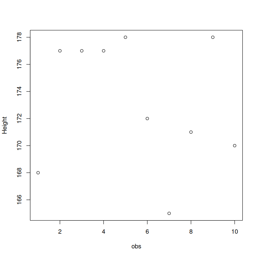
A matrix can be visualised using the plot function.
M <- cbind(obs,Height,Weight,BMI) # Create a matrix
plot(M)
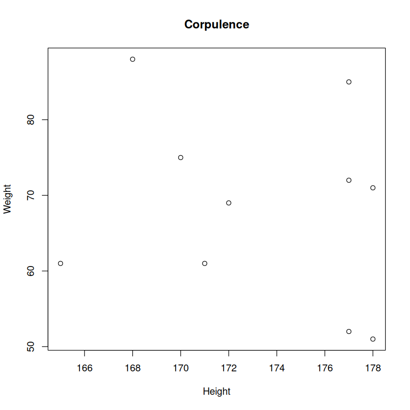
plot(Height,Weight,ylab="Weight",xlab="Height",main="Corpulence")
2.4.3. Arrays#
An array is composed of n dimensions where each dimension is a vector of R objects of the same type. An array of one dimension of one element may be constructed as follows.
x <- array(c(T,F),dim=c(1))
print(x)
[1] TRUE
The array x was created with a single dimension (dim=c(1)) drawn from the vector of possible values c(T,F). A similar array, y, can be created with a single dimension and two values.
y <- array(c(T,F),dim=c(2))
print(y)
[1] TRUE FALSE
A three dimensional array - 3 by 3 by 3 - may be created as follows.
z <- array(1:27,dim=c(3,3,3))
dim(z)
print(z)
- 3
- 3
- 3
, , 1

     [,1] [,2] [,3]
[1,]    1    4    7
[2,]    2    5    8
[3,]    3    6    9

, , 2

     [,1] [,2] [,3]
[1,]   10   13   16
[2,]   11   14   17
[3,]   12   15   18

, , 3

     [,1] [,2] [,3]
[1,]   19   22   25
[2,]   20   23   26
[3,]   21   24   27
is.matrix(z[,,1])
2.4.4. Exercise 4#
How would you access all of the elements in the second dimension of z ?
Show code cell source
z[,,3]
Show code cell output
| 19 | 22 | 25 |
| 20 | 23 | 26 |
| 21 | 24 | 27 |
2.4.5. Exercise 5#
What would you expect the output of the following code to be ?
print(z[,c(2,3),c(2,3)])
Show code cell output
, , 1

     [,1] [,2]
[1,]   13   16
[2,]   14   17
[3,]   15   18

, , 2

     [,1] [,2]
[1,]   22   25
[2,]   23   26
[3,]   24   27
Arrays need not be symmetric across all dimensions. The following code creates a pair of 3 by 3 arrays.
w <- array(1:18,dim=c(3,3,2))
print(w)
, , 1

     [,1] [,2] [,3]
[1,]    1    4    7
[2,]    2    5    8
[3,]    3    6    9

, , 2

     [,1] [,2] [,3]
[1,]   10   13   16
[2,]   11   14   17
[3,]   12   15   18
Objects of the vectors composing the array must be of the same type, but they need not be numbers.
u <- array(c(T,F),dim=c(3,3,2))
print(u)
, , 1

      [,1]  [,2]  [,3]
[1,]  TRUE FALSE  TRUE
[2,] FALSE  TRUE FALSE
[3,]  TRUE FALSE  TRUE

, , 2

      [,1]  [,2]  [,3]
[1,] FALSE  TRUE FALSE
[2,]  TRUE FALSE  TRUE
[3,] FALSE  TRUE FALSE
2.4.6. Exercise 6#
Try evaluating the following code. What would you expect the output to be ? Were you correct ?
z <- array(1:27,dim=c(3,3,3))
is.matrix(z)
is.matrix(z[,,1])
Show code cell output
2.5. Lists#
A list is a collection of R objects. list creates a list. unlist transform a list into a vector. The objects in a list do not have to be of the same type or length.
x <- c(1:4)
y <- FALSE
z <- matrix(c(1:4),nrow=2,ncol=2)
myList <- list(x,y,z)
print(myList)
[[1]]
[1] 1 2 3 4

[[2]]
[1] FALSE

[[3]]
     [,1] [,2]
[1,]    1    3
[2,]    2    4
Lists have very flexible methods for reference
by index number :
Notice the use of [[ ]]
a <- list()
a[[1]] = "A"
print(a)
a[[2]]="B"
print(a)
[[1]]
[1] "A"
[[1]]
[1] "A"

[[2]]
[1] "B"
by name
a$fruit = "Apple"
a$color = "green"
print(a)
[[1]]
[1] "A"

[[2]]
[1] "B"

$fruit
[1] "Apple"

$color
[1] "green"
Lists are recursive data structres !!
a <- list()
a[[1]] <- "hello"
a[[2]] <- list(c(1,2,3))
a[[2]]$message <- "hi !!"
print(a)
[[1]]
[1] "hello"

[[2]]
[[2]][[1]]
[1] 1 2 3

[[2]]$message
[1] "hi !!"
2.5.1. Exercise 6#
What would you expect the output of the following to be ?
print(a[[2]][[2]])
Show code cell output
[1] "hi !!"
print(a[[2]][[1]][2])
Show code cell output
[1] 2
print(a[2])
Show code cell output
[[1]]
[[1]][[1]]
[1] 1 2 3

[[1]]$message
[1] "hi !!"
print(a[[2]])
Show code cell output
[[1]]
[1] 1 2 3

$message
[1] "hi !!"
Confused !! Not surprising. Lists are recursive and inhomogenous - a tricky combination !! The key thing here is that [[ ]] returns a single item from a list and [ ] returns a list containing the elements indicated in the [ ]. For example
x <- list(1:3, "a", 4:6,list(4,5,6)) # x is a list with three items
x[1:2] # this prints a LIST containg the the first 2 items of list x
x[[2]] # this is the second ITEM contained in x - in this case, this is NOT a list
x[[4]] # this returns the fourth ITEM in the list x, which happens to be a list
x[4] # this returns a LIST containg the fourth item x - which is a LIST !! i.e x[4] is a list containing a list
-
- 1
- 2
- 3
- 'a'
- 4
- 5
- 6
- 4
- 5
- 6
If you are still confused - take a look at the following link to a useful section of Advanced R by Hadley Wickham.
2.5.2. Exercise 7#
What is a recursive data structure ? Do you know of any other types of recursive data structures other than a list ?
2.6. Data frames#
A dataframe has been referred to as “a list of variables/vectors of the same length”. In the following example, a dataframe of two vectors is created, each of five elements. The first vector, v1, is composed of a sequence of the integers 1 through 5. A second vector, v2, is composed of five logical values drawn of type T and F. The dataframe is then created, composed of the vectors. The columns of the data frame can be accessed using integer subscripts or the column name and the $ symbol.
v1 <- 1:5
v2 <- c(T,T,F,F,T)
df <- data.frame(v1,v2)
print(df)
df[,1]
df$v2
  v1    v2
1  1  TRUE
2  2  TRUE
3  3 FALSE
4  4 FALSE
5  5  TRUE
- 1
- 2
- 3
- 4
- 5
- TRUE
- TRUE
- FALSE
- FALSE
- TRUE
The dataframe may be created directly. In the following code, the dataframe is created - naming each vector composing the dataframe as part of the argument list.
df <- data.frame(foo=1:5,bar=c(T,T,F,F,T))
print(df)
  foo   bar
1   1  TRUE
2   2  TRUE
3   3 FALSE
4   4 FALSE
5   5  TRUE
Note - the rows of a data frame can be inhomogenous, the columns are homogenous.