4. Functions#
4.1. Using functions#
R comes with many many functions, and an ever growing and readily available collection of packages extends this number even further. You can get information on a function by using the help function. You can also see the “code” of the function.
4.1.1. Example 1 - Viewing a functions code using the functions name#
The function code for the ls (list) function can just be printed using print.
print(ls)
function (name, pos = -1L, envir = as.environment(pos), all.names = FALSE,
    pattern, sorted = TRUE)
{
    if (!missing(name)) {
        pos <- tryCatch(name, error = function(e) e)
        if (inherits(pos, "error")) {
            name <- substitute(name)
            if (!is.character(name))
                name <- deparse(name)
            warning(gettextf("%s converted to character string",
                sQuote(name)), domain = NA)
            pos <- name
        }
    }
    all.names <- .Internal(ls(envir, all.names, sorted))
    if (!missing(pattern)) {
        if ((ll <- length(grep("[", pattern, fixed = TRUE))) &&
            ll != length(grep("]", pattern, fixed = TRUE))) {
            if (pattern == "[") {
                pattern <- "\\["
                warning("replaced regular expression pattern '[' by  '\\\\['")
            }
            else if (length(grep("[^\\\\]\\[<-", pattern))) {
                pattern <- sub("\\[<-", "\\\\\\[<-", pattern)
                warning("replaced '[<-' by '\\\\[<-' in regular expression pattern")
            }
        }
        grep(pattern, all.names, value = TRUE)
    }
    else all.names
}
<bytecode: 0x5e9373b48f28>
<environment: namespace:base>
4.1.2. Example 2 - Viewing a functions code using page#
A similar effect can be achieved using the page function.
page(ls)
A function can be “called” in several ways.
4.1.3. Example 3 - Calling a function#
Functions are usually just called using there name along with appropriate comma seperated arguments in parenthesis i.e ().
x<-2
sin(x)
4.1.4. Example 4 - Calling a function using “ “#
A function can be also called by quoting its name. This is only usually seen in conjunction with functional programming techniques or occasional to change the format for using binary operators, such as + and *.
"sin"(x)
Note - almost everything in R is a variable or a function. Don’t believe me ?
4.1.5. Example 5 - Calling binary operators using “ “#
"<-"(x,3.14)
print(x)
"="(x,2.17)
print(x)
[1] 3.14
[1] 2.17
4.1.6. Example 6 - All operators are functions.#
X<-c(1,2,3,4)
"["(X,3)
4.1.7. Example 7 - help is a function#
"help"(help)
4.2. Creating your own functions#
Of course, you can create your own functions. The general structure of an R function definition is
function(arguments)
    {
       statements
       return(statement)
    }
where arguments is a comma separated list of argument names that can be used in the statements that make up the definition of the function, and statement is a valid R expression.
A function definition can be assigned to a variable and the function used through using the variable.
4.2.1. Example 8 - A simple function definition#
add<-function(x,y)
    {
      z <- x+y
      return(z)
    }

add(5,7)
However, functions can be used anonymously.
4.2.2. Example 9 - An anonymous function#
(function(x,y) { return(x+y) })(4,5)
This anonymous style of function definition is useful in conjunction with Map and Reduce, as will be seen later.
A function does not have to have a return statement. If it does not, value of the last R expression to be evaluated is returned by the function.
4.2.3. Example 10 - Implicit return#
add<-function(x,y)
    {
      x+y
    }

add(6,9)
Nor do all functions have to have a pair of {}s.
4.2.4. Example 11 - No {}s#
add<-function(x,y) x+y

add(12,2)
However, using a return statement and {}s makes the intent of your code much clearer.
A function can have an anonymous variable, which can be useful in anomynous functions.
4.2.5. Example 12 - anonymous variable#
f<-function(.)
    {
       return(sin(.) + .)
    }

f(1)
4.3. Default argument values#
Function arguments can have default values.
4.3.1. Example 13 - Default arguments#
f<-function(x,y,z=2)
    {
       return(x+2*y+3*z)
    }

f(2,3)
And arguments can be explicitly assigned. This can make your code quite clear.
f(x=2,y=3,z=7)
And means that you can swap the order.
f(y=3,z=7,x=2)
But be careful !!
f<-function(x=3,y,z=2)
    {
       return(x+2*y+3*z)
    }
4.3.2. Exercise 1#
What do you expect the output of the following code examples to be ?
f(y=2)
Show code cell output
f(2)
Show code cell output
Error in f(2): argument "y" is missing, with no default
Traceback:

1. f(2)
f(z=6,4,5)
Show code cell output
4.4. Higher Order Functions#
Functions can take functions as arguments. When they do, they are some times referred to as higher order functions.
4.4.1. Exercise 2#
What will the following code do ?
g<-function(f)
    {
       return(f(5))
    }

g(sin)
Show code cell output
Functions can also return functions that are defined within another function. Functions that do this are often referred to as closures.
4.4.2. Exercise 3#
What will the following code do ?
h<-function(x)
    {
       g<-function(y)
           {
              return(x+2*y)
           }
       return(g)
    }

a<-h(3)
print(a)

print(a(5))
Show code cell output
function(y)
           {
              return(x+2*y)
           }
<environment: 0x5e9377822290>
[1] 13
4.4.3. Exercise 4#
Can you think of any use cases for closures ?
4.4.4. Example 13 - Closures#
You can be quite terse with closures. The following is equivalent to the function in exercise 3.
h <- function(x) function(y) x + 2*y
Using anonymous functions with Map and Reduce can be very expressive of your codes intent, because puts everything on one line.
4.4.5. Example 14 Anonymous functions with Map and Reduce#
X<-list(1,2,3,4)
Y<-list(5,6,7,8)
Z<-Map(function(x,y) sin(x)+2*cos(y),X,Y)
print(Z)
[[1]]
[1] 1.408795

[[2]]
[1] 2.829638

[[3]]
[1] 1.648925

[[4]]
[1] -1.047803
4.4.6. Exercise 5#
Write some example code that uses anonymous functions with Map and Reduce combined together in one expression.
Show code cell source
X<-list(1,2,3,4)
Y<-list(5,6,7,8)
Z<-Reduce(function(a,b) a-b,Map(function(x,y) sin(x)+2*cos(y),X,Y))
print(Z)
Show code cell output
[1] -2.021965
4.4.7. Exercise 6#
Write some code that is equivalent to the above but using some combination of for, repeat, and/or while.
4.5. Variable scope and functions#
In programming, the scope of a variable (or object) describes where in an overall program the variable is “visible”. This is to understand as it can easily lead to “mysterious” bugs if not controlled properly.
4.5.1. Exercise 7#
For each of the following code examples, predict what the output will be.
a <- 2
f <- function(x)
    {
       return(a*x)
    }
f(5)
a<-6
f(5)
Show code cell output
a <- 2
f <- function(x)
    {
       a <- 7
       return(a*x)
    }
f(5)
print(a)
Show code cell output
[1] 2
a <- 2
f <- function(x)
    {
       a <<- 7
       return(a*x)
    }
f(5)
print(a)
Show code cell output
[1] 7
4.5.2. Exercise 8#
Using just a few sentences, can you describe why the output is what is as it is in each of the code examples in exercise 7.
4.6. Currying functions#
Sound alikes.
Curry - a popular dish | Curry - a computer scientist
| -
 |
| 
One use of closures is to “freeze” the value(s) of one or more arguments of a function. This can be useful when passing functions to other functions and is often required when using, for example, optimisers to maximise likelihood functions.
4.6.1. Example 15#
# Function to be optimised with respect to x for a given set of paramaters a,b, and c
g <- function(x,a,b,c)
       {
          return(a*x*x+b*x+c)
       }

a <- 4
b <- 3
c <- 1
f <- function(x)
    {
      return(g(x,a,b,c))
    }
4.6.2. Exercise 9#
What will the output of the following be ?
f(7)
Show code cell output
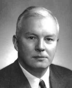
This technique is useful - but it does not generalise very well. However, it is possible to create a function that takes a function, along with the arguments to “freeze” , and which produces a new function with just the “unfrozen” arguments. This process is often called “currying” the function, and the new function referred to as the “curried” function. These terms are named after one of the first computer scientists to consider, study, use and champion functional programming techniques - Haskell B Curry. Incidentally, he also has a (functional) programming language named after him - Haskell.
## a function to help automate the "freezing" of the parameters

curry <- function(func,...)
    {
       return (function(.) return(func(.,...)))
    }
4.6.3. Example 16#
f <- curry(g,4,3,1)
f(7)
4.6.4. Exercise 10#
What is the advantage of the code in Example 16 when compared to that in Example 15 ?
It does not use global variables.
However, currying is a pretty standard functional programming technique. So the curry function has already been implemented, (several times), in packages on CRAN.
4.6.5. Exercise 11#
Install the functional package from CRAN and have a look at what methods it offers. Try using the Curry function in the package to redo Example 16.
